by David Manthey (manthey@orbitals.com)
Copyright 1999-2005 by David Manthey
A PDF version of this paper is available here: LEAST.PDF
Introduction
List of Symbols
General Technique
Potential Problems
Linear Technique
Error Residuals, Ellipsoids, and Confidence
An Example Problem
A Linear Solution
A Nonlinear Solution
An Error Ellipse
References
The method of least squares is used to solve a set of linear equations having more equations than unknown variables. Since there are more equations than variables, the solution will not be exactly correct for each equation; rather, the process minimizes the sum of the squares of the residual errors. The method is very powerful and can be applied to numerous applications.
In the general case, the least-squares method is often used to solve a set of non-linear equations that have been linearized using a first-order Taylor-series expansion. Solving non-linear equations is an iterative process using Newton’s method. The speed of convergence is dependent on the quality of an initial guess for the solution. The non-linear least-squares method is often referred to as a bundle adjustment since all of the values of an initial guess of the solution are modified together (adjusted in a bundle). This technique is also occasionally referred to as the Gauss-Newton method.
The least-squares method is not new; Legendre invented the method is 1805, and reference books have mentioned least squares in their titles as early as the 1870s. However, in most books about least squares, the general method is bound inextricably with the book's primary subject matter. There is little uniformity between different books, or even within a single book, on the designation of different variables. This makes it difficult to understand the method. This paper provides a new description of least squares which hopefully describes the process in a simple and straight-forward manner. A complete derivation of the method is not provided, only a functional description. Familiarity with matrices and partial derivatives is assumed.
An example problem is provided, computing the location of a circle based on a set of points. The example shows a linear solution and an iterative nonlinear solution to this problem as well as some error analysis.
| ai | coefficients of a linear equation |
| e | relative size of adjustment compared to initial value |
| Fi(x1,x2,x3,...) | equation based on a set of unknowns. This is not necessarily a function. The equation must be solved for the value (i.e., Fi(x1,x2,x3,...)=ki) whose error will be minimized |
| Fisher(a,v1,v2) | the Fisher distribution |
| J | the Jacobian matrix. This is the partial differentials of each equation with respect to each unknown. Sometimes written
J= |
| K | vector of residuals. Each component is the difference between the observation, ki, and the equation evaluated for the initial guess, xi0 |
| ki | an observation. The least-squares process minimizes the error with respect to the observations |
| N | the normal matrix. N=JtWJ |
| Q | cofactor matrix. The inverse of W. This is typically the standard deviations of the measurements |
| Qxx | the covariance matrix. Also called the variance-covariance matrix. Qxx=N-1 |
| Q'xx | a sub-matrix of the covariance matrix. Used to calculate an error ellipse |
| qxxij | a value within the covariance matrix |
| r | the degrees of freedom. This is the number of equations minus the number of unknowns |
| S02 | the reference variance. This is used to scale the covariance matrix |
| Saxis | length of the semi-axis of an error ellipse based on the covariance matrix |
| Saxis% | length of the semi-axis of an error ellipse with a specific confidence level |
| W | weighting matrix. This is a square symmetric matrix. For independent measurements, this is a diagonal matrix. Larger values indicate greater significance |
| wi | the diagonal components of the weighting matrix |
| X | vector of initial guesses for the unknowns |
| X' | vector of refined guesses for the unknowns. X'=X+DX |
| xi | an unknown value. This is solved for in the least-squares process |
| x'i | the refined guess for an unknown value. x'i=xi0+Dxi |
| xi0 | the initial guess for an unknown |
| DX | vector of adjustment values. The initial guesses are adjusted by this amount |
| Dxi | an adjustment value. This is added to the initial guess to improve the solution |
| G(v) | the Gamma distribution |
The general least squares process can be used to solve a set of equations for a set of unknowns. The only requirement is that there are at least as many equations as there are unknowns.
If the equations are linear, the least-squares process will produce a direct solution for the unknowns. If the equations are not linear, an initial guess of the unknowns is required, and the result is an adjustment to the initial parameters. This is repeated until the results converge (the adjustments become very close to zero). The linear case is an adjustment using zero as the initial guess of all parameters.
The process requires a set of equations with the unknowns on one side and some known quantity on the other. Let xi be the set of unknowns, and let the equations be of the form
Fi(x1,x2,x3,...)=ki
where ki is the observation (value) whose least-squares error will be minimized. Since there are more equations than unknowns, the solution of the unknowns will not be exact. Using the solution to compute the equation, Fi(x1,x2,x3,...), will not generate the exact observation value, ki. The square of the difference between the evaluated equation and the observation is minimized.
There is typically one equation for each observation. In photogrammetry, this might be one equation for each x pixel coordinate and one equation for each y pixel coordinate. Each equation is not required to have all of the unknowns in it.
The Jacobian matrix, J, is the matrix of the partial differentials of each equation with respect to each unknown. That is,
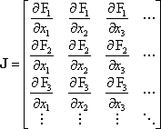
In general, the height of the Jacobian matrix will be larger than the width, since there are more equations than unknowns.
Furthermore, let the vector K be the vector of the residuals. A residual is the difference between the observation and the equation calculated using the initial values. That is

One further parameter is a weighting matrix, W. This is a matrix which includes the expected confidence of each equation and also includes any dependence of the equations. A larger value in the weighting matrix increases the importance of the corresponding equation (larger values indicate greater confidence). It is a square symmetric matrix with one row per equation. The main diagonal contains the weights of the individual equations, while the off-diagonal entries are the dependencies of equations upon one another. If all of the observations are independent, this will be a diagonal matrix. The cofactor matrix, Q, is the inverse of the weighting matrix (i.e., Q=W-1).
Let xi0 be an initial guess for the unknowns. The initial guesses can have any finite real value, but the system will converge faster if the guesses are close to the solution. Also, let X be the vector of these initial guesses. That is

It is desirable to solve for the adjustment values, DX. This is the vector of adjustments for the unknowns

where, based on the initial guess, X, and an adjustment, DX, a set of new values are computed
X'=X+DX
To solve for DX, (see the references for the reasoning behind this solution)
DX=(JtWJ)-1JtWK
In various texts, the normal matrix, N, is defined as
N=JtWJ,
and the covariance matrix (sometimes referred to as the variance-covariance matrix), Qxx, is defined as
Qxx=(JtWJ)-1=N-1
If the weighting matrix is diagonal, then DX can be solved by row reduction of the matrix

where w1, w2, w3, ... are the diagonal elements of the weighting matrix. Note that the left side of the matrix is the normal matrix, N.
The initial guesses, xi0, are updated using the solution of the adjustment matrix, DX, as follows
X'=X+DX
or
x'i=xi0+Dxi
The process is repeated using the new values, x'i, as the initial guesses until the adjustments are close to zero.
Practically, an adjustment is close to zero when it is small compared to the absolute magnitude of the value it is adjusting, i.e., Dxi < xi0 e, where e is a small value. The actual value for e can be selected based on the number of decimal digits of precision used in the calculations. Typically, the order of magnitude of e will be a few less than the number of digits of precision. For example, if the calculations are done on a computer using standard double precision (8-byte) values, the computer can hold around 15 digits of precision; therefore e is about 10-12.
There are conditions where the solution will not converge or will converge to undesirable values. This process finds a local minimum. As such, there may be a better solution than the one found. A solution is dependent on the equations, Fi(x1,x2,x3,...), being continuous in x1,x2,x3,.... The first and second derivatives do not need to be continuous, but if the equations are not continuous, there is no guaranty that the process will converge. Also, in certain circumstances, even if the equations are continuous, the solution may not converge. This can happen when the first and second derivatives of the equations have significantly different values at the initial values than at the solution.
In any case where the solution does not converge, a solution may still be able to be obtained if different starting values, xi0, are used.
For sets of linear equations, the least-squares process will produce a direct solution for the unknowns. The linear case is mathematically the same as the general case where an adjustment is performed using zero as the initial guess of all parameters. Only a single iteration is required for convergence.
The equations must be of the form
Fi(x1,x2,x3,...)=a1x1+a2x2+a3x3+...=ki
The Jacobian matrix, J, is therefore

where aij is the ith coefficient of the jth equation.
Since the initial guesses are all zero, the vector of residuals, K, is

If the weighting matrix is diagonal, then DX can be solved by row reduction of the matrix

The final solution will be the adjustment values. That is
X=DX
or
xi=Dxi
The covariance matrix, Qxx, contains the variance of each unknown and the covariance of each pair of unknowns. The quantities in Qxx need to be scaled by a reference variance. This reference variance, S02, is related to the weighting matrix and the residuals by the equation
![]()
where r is the number of degrees of freedom (i.e., the number of equations minus the number of unknowns).
For any set of quantities, an error ellipse can be calculated. The dimensions and orientations of the ellipse are calculated from the coefficients of the covariance matrix. Only the coefficients of the covariance matrix in the relevant rows and columns are used. This is the appropriate n x n sub-matrix, where n is the number of dimensions for the error ellipse. The sub-matrix is symmetric.
The ellipse matrix is composed of entries from the covariance matrix. For example, a three-dimensional error ellipsoid is computed from

where qxxij are values from the covariance matrix Qxx, and a, b, and c are the indices for the unknowns for which the ellipse is computed.
The error ellipse semi-axes are given by
![]()
The orientation of the error ellipse is the column eigenvectors of Q'xx.
To determine the error to a specific confidence level, the length of the semi-axis is multiplied by a confidence factor based on the Fisher distribution using the formula
![]()
where the confidence is a number from 0 to 1, with 1 being complete confidence, and r is the number of degrees of freedom. The Fisher distribution is determined from the equation
![]()
where the Gamma function, G(v), is given by
![]()
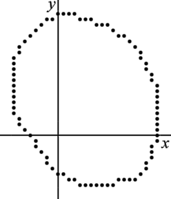
Given a set of two-dimensional points, find the circle best represented by these points.
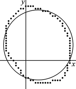
For this example, there are 82 points, see also the figure to the right:
| 3,-8 | 4,-9 | 5,-9 | 6,-9 | 7,-9 | 8,-9 | 9,-9 | 10,-9 | 11,-8 | 12,-8 |
| 13,-8 | 14,-8 | 15,-7 | 16,-6 | 16,-5 | 17,-4 | 17,-3 | 17,-2 | 18,-1 | 18,0 |
| 18,1 | 18,2 | 18,3 | 18,4 | 18,5 | 18,6 | 18,7 | 18,8 | 18,9 | 17,10 |
| 17,11 | 16,12 | 16,13 | 15,14 | 15,15 | 14,16 | 13,17 | 12,18 | 11,18 | 10,19 |
| 9,20 | 8,20 | 7,20 | 6,21 | 5,21 | 4,21 | 3,22 | 2,22 | 1,22 | 0,22 |
| -1,21 | -2,21 | -3,20 | -4,19 | -5,18 | -6,17 | -7,16 | -7,15 | -8,14 | -8,13 |
| -8,12 | -8,11 | -8,10 | -8,9 | -8,8 | -8,7 | -8,6 | -8,5 | -8,4 | -7,3 |
| -7,2 | -6,1 | -5,0 | -4,-1 | -4,-2 | -3,-3 | -2,-4 | -2,-5 | -1,-6 | 0,-7 |
| 1,-7 | 2,-8 |
Let the points be denoted (xi,yi). That is, (x1,y1)=(3,-8), (x2,y2)=(4,-9), (x3,y3)=(5,-9), , ...
A circle can be defined by the equation
![]()
where (x0,y0) is the center of the circle and r is the radius of the circle.
Ideally, it is desirable to minimize the square of the distance between the points defining the circle and the circle. That is, minimize
![]()
This is equivalent to performing the least-squares process using the equations
![]()
The equation of a circle is not linear in the unknown values x0, y0, and r. The equation of a circle can be written in the linear form
A(x2+y2)+Bx+Cy=1
where
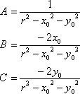
This can be rewritten for the original unknowns as
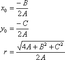
Note that by using the linear form of the circle equation, the square of the distance from each point to the circle in not the value that is being minimized.
Using the equation A(x2+y2)+Bx+Cy=1 with the unknowns A, B, and C, the Jacobian matrix is
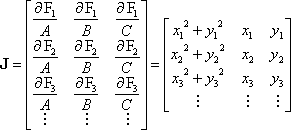
Placing numerical values in the Jacobian matrix gives

Since all initial guesses are zero, the residual vector is

Lacking other information, the weighting matrix, W, is the identity matrix. That is
W=I
The unknowns, A, B, and C, can be solved for using the equation
X=(JtWJ)-1JtWK=(JtJ)-1JtK
This can be simplified to

Numerically, this is

Solving for the unknowns, this is


Solving for the circle parameters, this is
x0=4.778760172
y0=5.875467325
r=14.67564038
This solution is shown superimposed on the original points in the figure to the right. Note that the circle does not fit the data points very well because the solution used the linear form of the circle equations. A much better fit can be obtained using the nonlinear equations.
Instead of solving for the linear parameters, A, B, and C, it is more desirable to solve for the values x0, y0, and r using an equation that minimizes the distance from the points to the circle. The following equation is used
![]()
The Jacobian matrix is
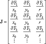
where
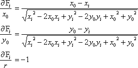
The solution of x0, y0, and r will require multiple iterations. A starting guess for these values is required. The starting guess can be arbitrary provided the equations are valid. A starting guess of
x0=0
y0=0
r=15
will be used.
Placing numerical values in the Jacobian matrix gives

The residual vector is
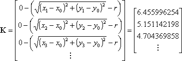
Again, lacking other information, the weighting matrix, W, is the identity matrix.
The adjustments of the unknowns, Dx0, Dy0, and Dr, can be solved for using the equation
DX=(JtWJ)-1JtWK=(JtJ)-1JtK
Numerically, this is

Solving for the adjustment values, this is

The circle parameters are then adjusted to
x0'=x0+Dx0=0+6.134768609=6.134768609
y0'=y0+Dy0=0+6.649105121=6.649105121
r'=y+Dr=15+-2.364891088=12.63510891
This new solution is now used to compute a new Jacobian matrix and a new residual vector, which are then used to again solve for DX. The next iteration is

The circle parameters are now adjusted to
x0'=x0+Dx0=6.134768609+-1.033761936=5.101006672
y0'=y0+Dy0=6.649105121+-0.4464161055=6.202689015
r'=y+Dr=12.63510891+1.584613997=14.21972290
Additional iterations are performed until the adjustment values become close to zero. When performing computations with ten significant figures, after nine iterations, the values have converged to
x0=5.155701836
y0=6.233137797
r=14.24203182
This solution is shown superimposed on the original points in the figure to the right. Note that the circle fits the data points significantly better than the linear solution.
To determine the expected error of the nonlinear solution of the circle, the error ellipse can be calculated. To illustrate this, the error ellipse of the circle’s center will be computed.
The error ellipse is computed using the covariance matrix

Since only the error ellipse for the center of the circle, (x0,y0), is desired, the matrix of interest is
![]()
The matrix Q'xx is composed of the entries in the first two columns and rows of the matrix Qxx since x0 corresponds to the first column and y0 to the second column of the Jacobian matrix.
The eigenvalues of Q'xx are
![]()
The eigenvectors specify the orientation of the ellipse. The eigenvectors are
![]()
The reference variance is computed based on the residual matrix and on the degrees of freedom. The number of degrees of freedom is the number of observations (82 observations – the number of points used to compute the circle) minus the number of unknowns (3 unknowns - x0, y0, and r). The reference variance is
![]()
The error ellipse can be computed for any confidence level. The Fisher distribution needs to be computed for the selected confidence. Although the reference variance was computed based on the total number of unknowns, the Fisher distribution is computed only for the number of unknowns in the ellipse. For 95% confidence
Fisher(1-0.95,2,79)=3.11227
Based on this information, the semi-axes of the error ellipse are
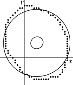

The 95% confidence error ellipse is shown on the same graph as the circle, see figure to the right. The error ellipse has been magnified by a factor of 5 to make it more visible.
The meaning of the 95% confidence error ellipse is that if more points are added to improve the calculation of the circle, there is 95% probability that the center of the circle will remain within the area specified by the ellipse. As expected, as more points are used to compute the circle, the area of the ellipse becomes smaller. If the points lie closer to the actual circle, this will also reduce the ellipse area.
[1] Nash, Stephan G. and Sofer, Ariela, Linear and Nonlinear Programming, McGraw-Hill Companies, Inc, New York, 1996. ISBN 0-07-046065-5.
[2] Wolf, Paul R. and Ghilani, Charles D., Adjustment Computations, John Wiley and Sons, Inc, New York, 1997. ISBN 0-471-16833-5.